Histogramming and Binning Data with NumPy in Python

NumPy is a fundamental package for computing scientific-related things using Python. It provides powerful functionality for working with arrays and matrices that are well-optimized for speed and performance. NumPy can create histograms and bin data. These are important methods for exploring, summarizing, and visualizing the dataset’s distribution. This guide will explore “Histogramming and Binning Data with Numpy in Python” So let’s start

Data analysis often involves categorizing continuous data into discrete groups, a process known as binning. One of the most effective ways to visualize such grouped data is through histograms. Numpy library provided powerful tools to perform histogramming and binning efficiently.

What is Histogramming and Binning

Histogramming

A histogram is a graphical representation of the distribution of numerical data. It breaks the data into bins and counts how many values fall into each bin (intervals). This helps us to understand patterns, trends, and outliers in data.

Histograms are useful in statistical analysis, data visualization, and machine learning, as they provide insight into data distribution.

Key Properties of Histograms:

• Histograms illustrate how frequently data is distributed.
• The x-axis shows the variable of the data being analyzed.
• The y-axis indicates the count of data points (frequency) in each bin.

Binning

Binning is the process of dividing continuous data into a set of intervals. Each interval (bin) represents a range of values and the data points that fall within that range.

Histograms are built upon binning, and NumPy makes this process seamless with its numpy.histogram() function.

Creating Histograms with NumPy’s histogram() Method

NumPy provides the numpy.histogram() function, which computes the frequency distribution of a dataset.

np.histogram(a, bins=10, range=None, normed=False, weights=None, density=None)

Key parameters are:

• a: Input data array
• bins: Number of bins or specifying bin edges directly
• range: Data range tuple (min, max) to use for histogram
• normed: Normalize histogram to form a probability density
• weights: Optional array of weights for each data point
• density: Normalize histogram to integrate to 1

Let’s see some examples of using np.histogram() on both simulated and real-world data.

Example 1: Basic Histogram Example With Numpy

import numpy as np
import matplotlib.pyplot as plt

# Sample data
data = np.random.randn(1000)  # 1000 random numbers from a normal distribution

# Compute histogram
hist, bin_edges = np.histogram(data, bins=10)

print("Histogram Counts:", hist)
print("Bin Edges:", bin_edges)

Visualizing the Histogram with Matplotlib

plt.hist(data, bins=10, edgecolor='black')
plt.xlabel('Value')
plt.ylabel('Frequency')
plt.title('Histogram Example')
plt.show()

Understanding the Output

• hist: An array representing the count of values of each bin.
• bin_edge: The edges of the bins define the interval ranges.

Example 2: Analyzing Histograms of Iris Measurements

Let’s look at an example. We will load the Iris flower dataset. Then, we will compute histograms of the measurements. Next, we will analyze the distribution. Finally, we will plot the histograms.

from sklearn.datasets import load_iris
import numpy as np
import pandas as pd
import matplotlib.pyplot as plt

# Load data
iris = load_iris()
data = iris['data']

# Histogram of sepal length
sepal_length = data[:, 0]
counts, bin_edges = np.histogram(sepal_length, bins=15, density=True)

# Digitize sepal length values into bins
bins = np.digitize(sepal_length, bin_edges)

# Pandas DataFrame with binned data
df = pd.DataFrame({'sepal_length': sepal_length, 'bin': bins})

# Analyze binned data
print(df.groupby('bin').sepal_length.mean())

This enables us to examine and illustrate the distribution of sepal length values, providing valuable insights into the dataset. The analysis can also be broadened to include additional features.

Visualizing the Histogram with Matplotlib

# Plot histogram
plt.hist(sepal_length, bins=15, density=True)
plt.xlabel('Sepal length (cm)')
plt.ylabel('Probability density')
plt.show()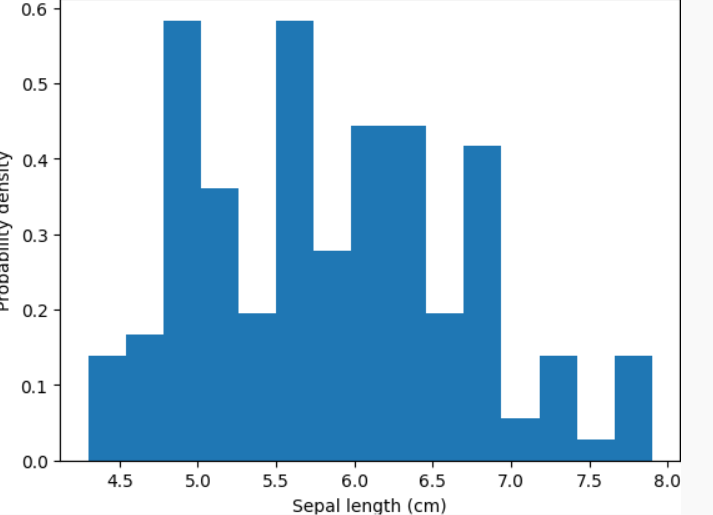

How to Choose the Optimal Bin Size

Bin size and range significantly impact the shape of the histogram. Here are some guidelines for selecting bin sizes:

• Scott’s normal reference rule – This method is more suitable for normal distributions. The bin width is calculated as (3.5 * std) / N^(1/3), where std denotes the standard deviation.
• Sturges’ formula – K = 1 + log2(N) provides a basic guideline. Here, N represents the number of data points, while K indicates the number of bins.
• Square root choice – The bin width is determined by sqrt(x_max – x_min) / sqrt(N). This approach is effective for smoother distributions.
• Freedman–Diaconis rule – The bin width is given by 2(IQR) / N^(1/3), with IQR representing the interquartile range of the data. This method is beneficial for handling outliers.
• Shimazaki and Shinomoto method – This technique optimizes dynamic bin widths by minimizing a cost function.
• In the end, domain knowledge should help choose the right method. It balances smoothing, overfitting, and showing true distribution patterns.

Automated methods like 'auto' and 'fd' in np.histogram() are also available.

Controlling Bins in NumPy Histograms

The number and size of bins significantly impact how the histogram represents data. NumPy allows fine-tuning of bins in different ways.

Adjusting the Number of Bins

The bins parameter controls the number of bins in the histogram method.

plt.hist(data, bins=20, edgecolor='black')  # Increase to 20 bins
plt.show()

Custom Bin Ranges

You can specify your bin ranges using a list:

custom_bins = [-3, -2, -1, 0, 1, 2, 3]
plt.hist(data, bins=custom_bins, edgecolor='black')
plt.show()

Using Bin Width Instead of Count

Instead of setting a fixed number of bins, you can define bin width.

bin_width = 0.5
bins = np.arange(min(data), max(data) + bin_width, bin_width)
plt.hist(data, bins=bins, edgecolor='black')
plt.show()

Real-World Use Cases of Histogramming

Some common use cases where histograms can provide valuable insights into data:

Understanding the Data Distribution

Histograms help in identifying skewness, normality, and outliers in datasets. Analysts can use them to detect patterns, making it easier to preprocess and clean the data.

Image Processing

Binning plays a crucial role in image processing, particularly in analyzing pixel intensity distributions. In computer vision, histograms help enhance images, detect edges, and segment objects effectively.

Financial Analysis

Financial analysts use histograms to study stock price fluctuations and market trends. By analyzing the frequency distribution of stock returns, traders can make informed decisions.

Machine Learning and AI

Histograms help in feature engineering by transforming continuous variables into categorical ones. Many machine learning models benefit from binned data to improve performance and accuracy.

Medical Data Analysis

In medical research, histograms help analyze patient data. This includes age distributions, disease occurrences, and treatments.

Related Blogs:

>> Procedural vs Object-Oriented Programming in Python

>> 5 Free Hosting Platforms for Python Applications

>> A Comprehensive Guide to Filter Function in Python

Conclusion: Histogramming and Binning Data with Numpy

Histogramming and Binning Data with NumPy in Python is essential for data analysis and visualization. With NumPy’s np.histogram() and Matplotlib’s plt.hist(), you can efficiently categorize and analyze data distributions.

Mastering histogramming in Python will enhance your data analysis skills and improve insights from numerical data.

I hope you understand this guide. If you have any questions about the article “Histogramming and Binning Data with Numpy,” feel free to comment.

Happy Coding!